Most manufacturers build their data warehouse the way they build their org chart — in silos. Operations gets its schema. Finance gets its schema. And somewhere in between, the CFO and the plant manager spend forty-five minutes on a call arguing about why the production cost numbers don’t match.
This isn’t a data quality problem. It’s an architecture problem.
A well-structured manufacturing data warehouse doesn’t just store operational and financial data — it reconciles them at the model layer so that a production efficiency metric and a cost-per-unit figure are speaking the same language, drawing from the same source of truth, and rolling up the same way. Getting there requires deliberate design decisions from the start. Here’s how to do it.
Start With the Business Question, Not the Source System
The most common mistake we see manufacturers make is designing their warehouse around what’s easy to extract rather than what leadership actually needs to answer. The ERP has a particular table structure. The MES has its own schema. The SCADA historian exports in a certain format. Teams build ingestion pipelines for each, load the data largely as-is, and call it a warehouse. What they’ve actually built is a data swamp with an ETL layer on top.
Before you write a single ingestion job, map out the twenty or thirty core questions your business asks repeatedly. These will typically span two domains:
Operations wants to know: Where is downtime concentrated? What is our actual OEE by machine and shift? Where are yield losses occurring? How does cycle time today compare to standard? Are we running to schedule?
Finance wants to know: What is our actual cost of production versus standard? How is labor efficiency trending by department? What are our scrap and rework costs? How do maintenance expenditures correlate with output? Where are the variances in our cost of goods manufactured?
These questions look different on the surface, but they share underlying data: machine run time, part counts, labor hours, material consumption. The warehouse architecture should reflect that shared foundation.
Build a Unified Conformed Dimensions Layer
The reason ops and finance so often produce conflicting numbers is that they’re slicing the same underlying reality along different dimension hierarchies. Finance rolls up by cost center. Ops rolls up by work cell. Neither maps cleanly to the other, so reconciliation happens manually in Excel — or not at all.
The fix is conformed dimensions. A conformed dimension is a shared, agreed-upon reference table that multiple fact tables join to, ensuring that “Plant 2, Line B, Shift 3” means exactly the same thing whether you’re looking at OEE data or labor variance data.
The core conformed dimensions for a manufacturing warehouse typically include:
Time — a standard date and shift dimension that captures calendar date, fiscal week, fiscal period, and shift designation. Both ops and finance need to aggregate by period; this dimension makes that aggregation consistent.
Location — a hierarchy from facility down through department, cost center, production area, work cell, and machine. Finance thinks in cost centers. Ops thinks in work cells. This dimension bridges them.
Product — a hierarchy from product family down through part number and revision. Finance needs this for cost rollups. Ops needs it for yield and throughput analysis. The SKU or part number is the join key.
Employee and Shift — for labor efficiency analysis, a shared employee dimension with department and shift assignment enables both HR cost allocation and operations productivity tracking to use the same underlying records.
Resource or Equipment — a master equipment list with asset ID, asset type, cost center assignment, and maintenance class. This is the link between maintenance expenditure (finance) and equipment availability (ops).
Without these conformed dimensions, you’re not building a warehouse — you’re building two separate data marts that happen to live in the same database.
Design Your Fact Tables Around Business Processes, Not Source Systems
Fact tables should represent business events, and manufacturing has a handful of core events that both ops and finance care about deeply. The most important are:
Production Orders — each row represents a production order or work order, with measures for quantity ordered, quantity produced, quantity scrapped, standard hours, actual hours, and standard material cost versus actual material cost. This fact table is the spine of manufacturing analytics. Ops uses it for throughput and yield. Finance uses it for production variance.
Machine Events — each row represents a time-stamped machine state change: running, idle, planned downtime, unplanned downtime. Measures include duration and affected quantity. Ops uses this for OEE. Finance uses it for understanding how equipment availability drives absorption.
Labor Transactions — each row represents a labor booking against a work order or cost center, with measures for hours worked, labor class, and cost. This bridges the HR and payroll systems to operations.
Inventory Movements — each row represents a material movement: issue to production, receipt from production, scrap, return. Measures include quantity and standard cost. Finance uses this for inventory valuation and COGS. Ops uses it for material efficiency.
Maintenance Work Orders — each row represents a maintenance activity, with measures for labor hours, parts cost, total cost, and downtime caused. This is one of the richest integration points between ops and finance and often the most neglected.
The critical design principle: each fact table should carry the foreign keys to all relevant conformed dimensions. A production order fact row should join to time, location, product, and equipment — even if ops doesn’t care about cost center and finance doesn’t care about work cell. That join capability is what makes cross-functional analysis possible without bespoke data wrangling.
Establish a Standard Cost Bridge
Standard costing is the language of manufacturing finance, and it creates a natural join between operational metrics and financial reporting. But only if the warehouse is designed to support it.
A standard cost bridge is a table that carries the official standard cost rates for each combination of product, resource, and time period: standard labor rate by labor class, standard machine rate by equipment type, standard material cost by part number and revision. These rates are typically managed in the ERP and should be loaded into the warehouse as a slowly changing dimension — preserving history so that you can correctly value production from six months ago using the rates that were in effect at the time.
With a standard cost bridge in place, ops metrics and finance metrics become directly comparable. Actual hours times standard labor rate gives you the labor efficiency variance in dollar terms. Actual material consumption times standard material cost gives you the material usage variance. These are numbers that both the plant controller and the operations manager can hold simultaneously without arguing about whose version is right.
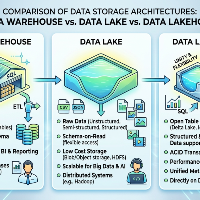
Separate Raw, Conformed, and Serving Layers
Manufacturing data comes from systems that weren’t designed to talk to each other. SCADA historians store millions of time-series readings. MES platforms track work orders and genealogy. ERPs hold financial transactions and master data. Quality systems log inspection results. Each has its own data model, its own export format, its own timestamp conventions, its own treatment of nulls and edge cases.
The warehouse architecture needs to absorb this messiness without letting it contaminate analytics. The standard approach is a three-layer model:
The raw layer captures source data exactly as it arrives. No transformations, no business logic, no joins. This is your audit trail and your recovery mechanism when something breaks downstream.
The conformed layer applies standardized transformations: timestamps normalized to a common timezone and grain, foreign keys resolved to the conformed dimension tables, business rules applied (how do we classify a five-minute stoppage — planned or unplanned?), and outliers flagged. This is where the heavy data engineering work happens, and it’s where ops and finance agree on definitions.
The serving layer builds the aggregations, metrics, and presentation models that feed dashboards and reports. OEE by work cell and shift. Cost variance by product and period. Maintenance cost per unit of output. These models are built on top of the conformed layer, which means they’re drawing from the same resolved reality.
This separation matters because ops teams and finance teams often have different latency needs. Operations may need near-real-time machine event data. Finance needs accurate period-end closes, not necessarily sub-hourly updates. A well-structured warehouse can serve both by maintaining high-frequency raw ingestion while running conformed and serving layer transformations on a schedule appropriate to each use case.
Governance Is Part of the Architecture
One of the most overlooked aspects of building a manufacturing data warehouse is metric governance. A warehouse that produces twenty-seven different versions of OEE — one per dashboard, each with slightly different exclusion rules — is not a warehouse. It’s a disagreement stored in a database.
Every key metric should have a single authoritative definition, documented and version-controlled: what time losses count as planned downtime? What quality threshold defines a scrap event versus a rework? How are partial shifts treated in efficiency calculations? These definitions should live alongside the code that implements them, and changes to them should go through a change control process that notifies both ops and finance stakeholders.
In practice, this means building metric definitions into your conformed layer as explicit, named, tested transformations — not as calculated fields buried inside a BI tool that only one analyst knows how to find.
The Payoff: A Conversation That Doesn't Require a Translator
When a manufacturing data warehouse is built this way, something changes in the organization. The CFO and the VP of Operations stop arguing about whose numbers are right, because there’s only one set of numbers. Finance can drill into a cost variance and see the specific work orders, shifts, and machines that drove it. Operations can see the dollar impact of downtime events, not just the hours. The weekly production review becomes a shared conversation about the same underlying reality, rather than a negotiation between two departments with competing spreadsheets.
That’s the real return on investment from getting the architecture right. Not faster dashboards. Not prettier reports. A company that can actually make decisions based on data it trusts.